About

This site documents a natural language processing (NLP) group project done in collaboration with rogerchenrc and laviniafr. In this we tested different NLP techniques and model architectures to create a CI/CD pipeline to train and deploy a multi-label classifier. The classifier was trained on dataset of movie descriptions to predict the top fitting genre(s) with 12 possible values including: Drama, Comedy, Action, Crime, Thriller, Romance, Horror, Adventure, Mystery, Family, Fantasy and Sci-Fi. The state of the best trained model was then saved to file and deployed on a custom built web server as demonstrated in the video below:

Data

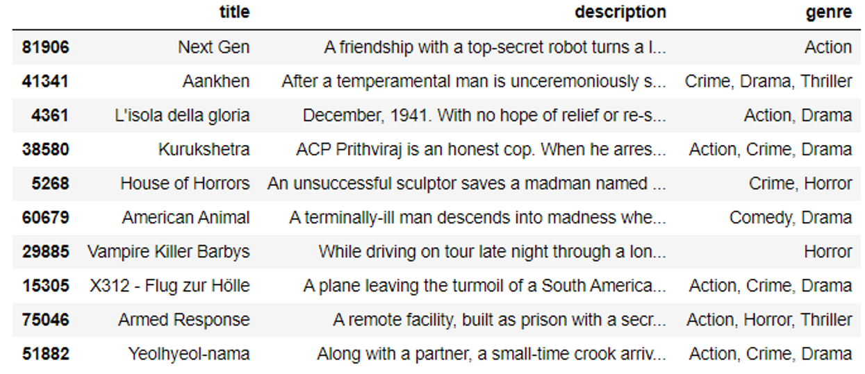
We decided to use the IMDb movies extensive dataset from Kaggle. This contains 84,983 samples providing a sufficient number to train a robust classifier. Although each film has many attributes, such as year of release and director, we only required the original title, description and list of genres to use as training labels. Some pre-processing was therefore required to remove samples missing this information and to remove unnecessary attributes. This lead to 2,115 samples being dropped with 83,740 remaining.

Analysing the Labels and Descriptions

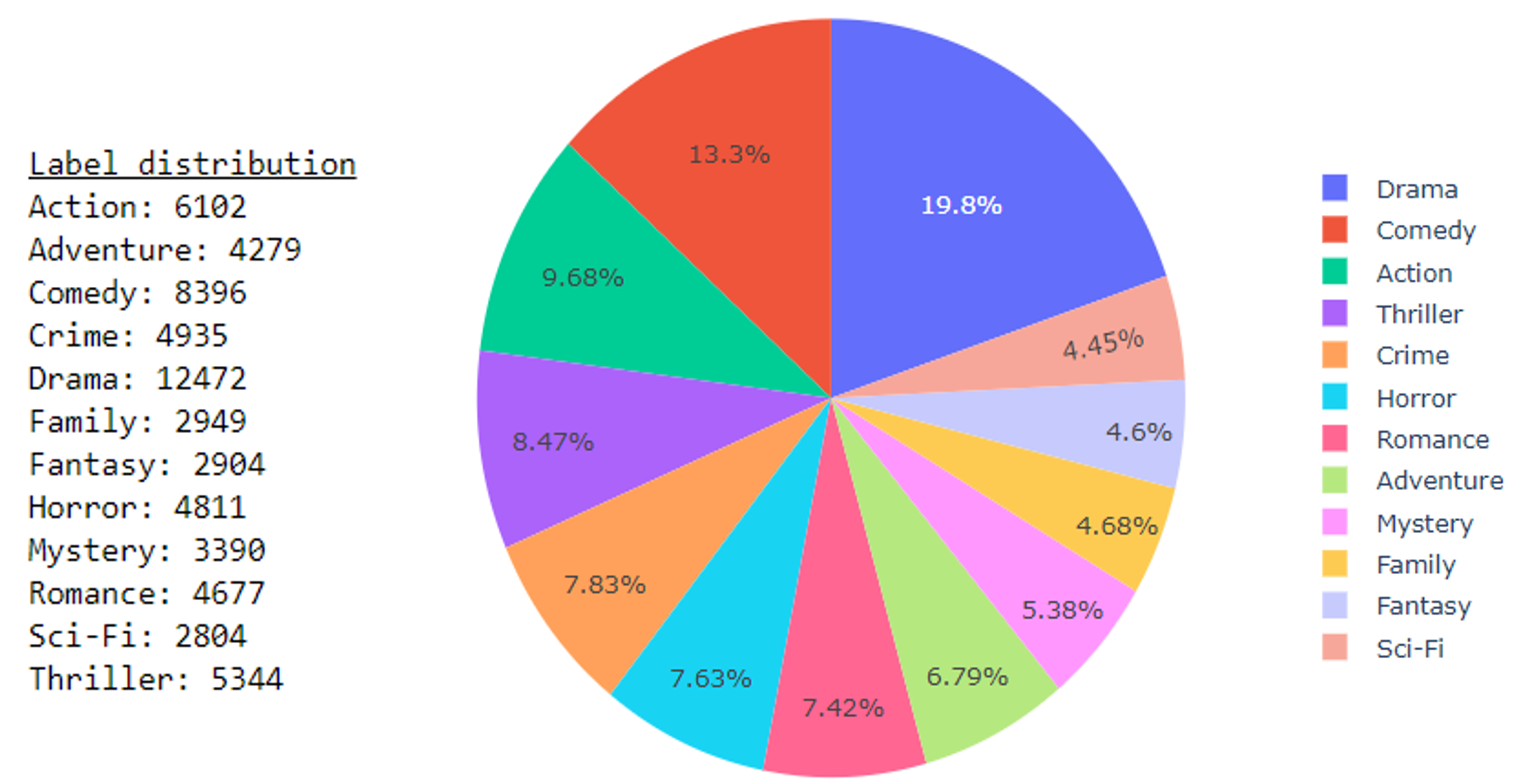
All films have between one and three genres, each of which can be used as a label during classification. After analysing all samples, it was discovered that there were 25 unique values. However, they were not evenly distributed with 26.7% of samples belonging to Drama and eight genres with less than 1%.

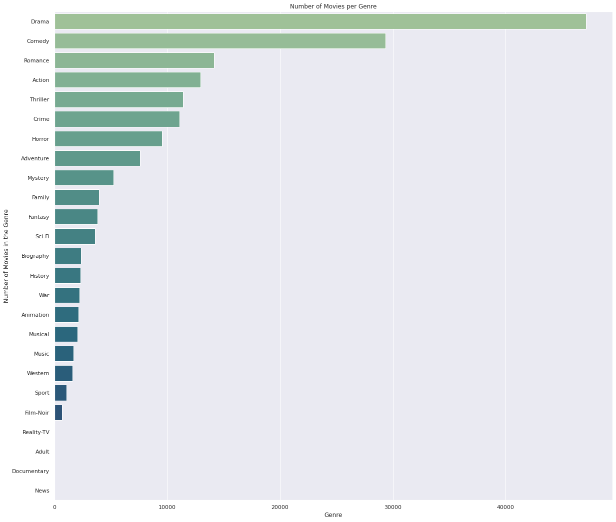
Figure 2a: Graph showing the number of samples belonging to each genre

As not all genres have enough representative samples, we initially decided to only keep the most common seven (although later extended to 12). After stripping the uncommon labels and dropping samples that no longer belonged to least one genre, we then evened up the label distributions through sampling. This is because an unbalanced label distribution can lead to bias when training a neural network.

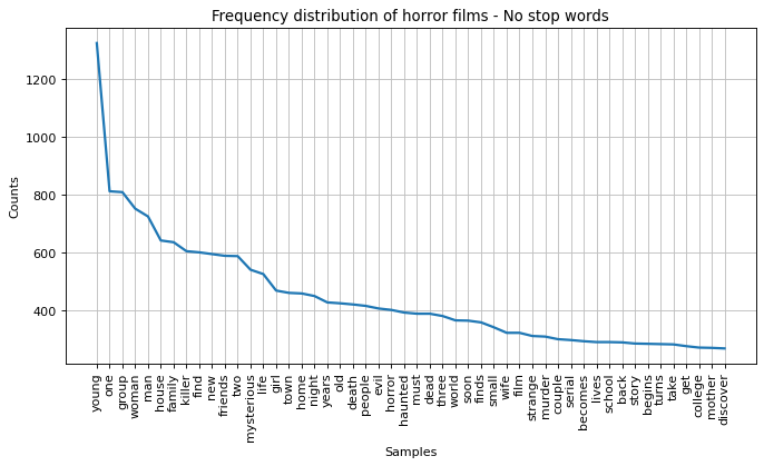
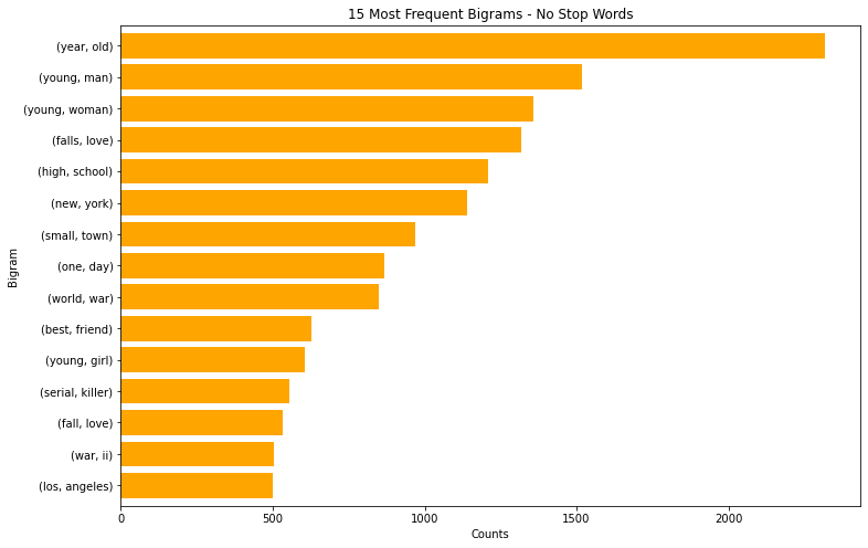
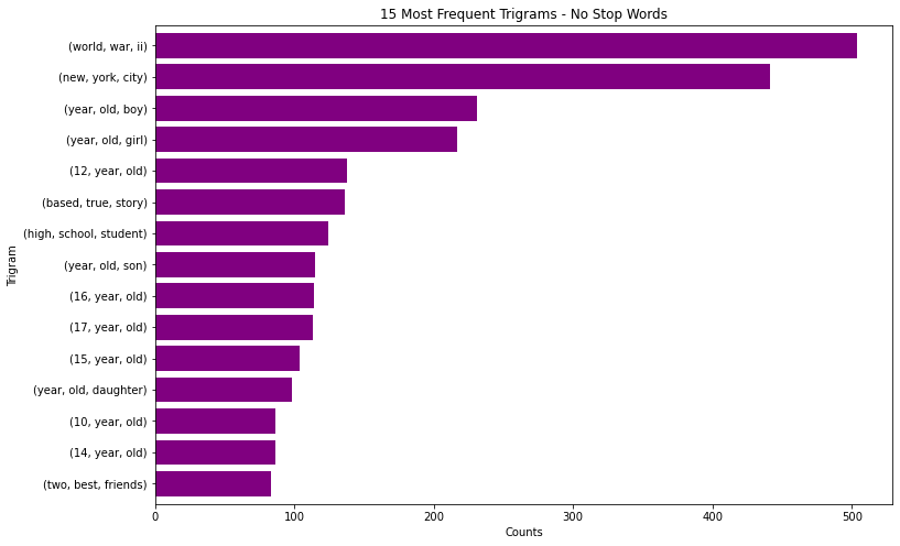
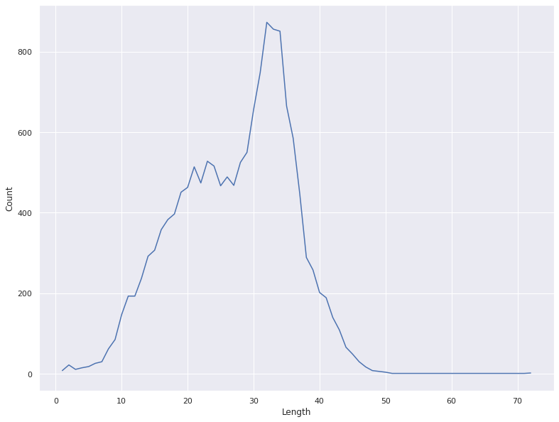
Figure 3a: Pie chart of label distribution across all samples

We used various methods to inspect the movie description text including: finding words that are representative of each genre, locating common stop words (e.g. a, the, for) as well as words consistently used across all descriptions (e.g. young, man) that are common across all genres, discovering the most frequent bigrams and trigrams and viewing the number of words in each description.

Figure 4a: Scattertext graph of word frequencies for horror film descriptions

Label Encoding and Text Processing

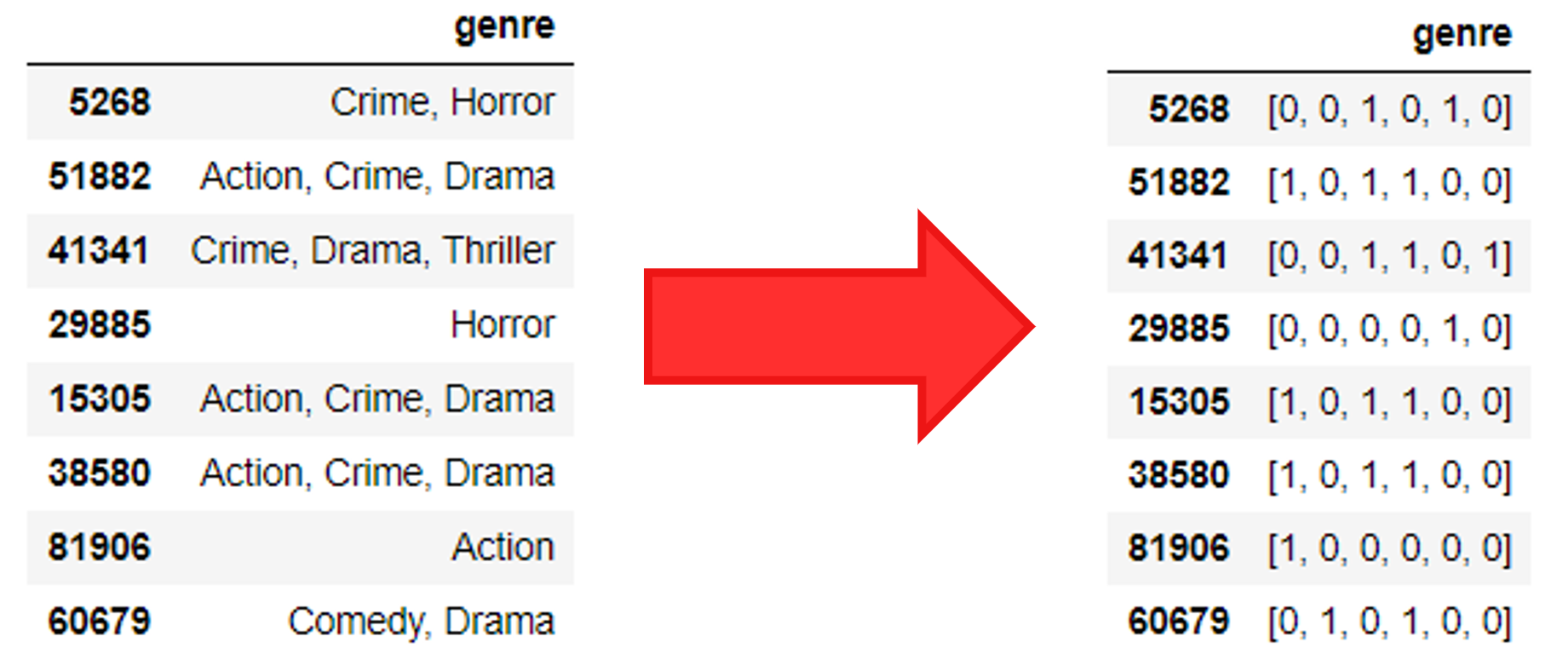
Each film has between one and three genres allowing us to perform multi-label classification. Unlike multi-class, where only one output is given, multi-label allows multiple predictions to be made at once. Therefore to represent the multiple combinations of labels in a way that the classifier can understand, we used multi-hot encoding, i.e. a binary representation, where 1 signifies that a description belongs to a genre and 0 means that it does not.

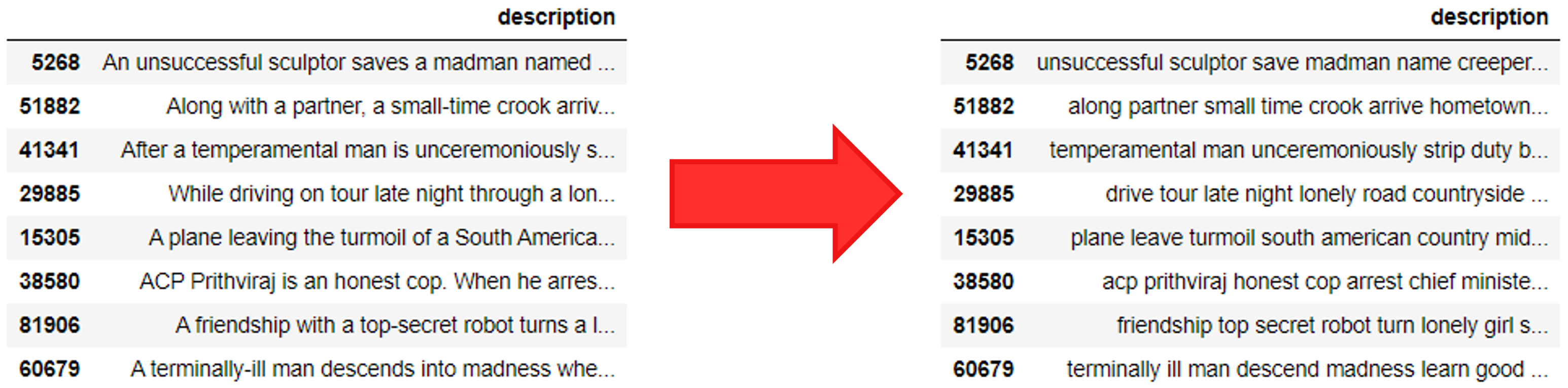
Figure 5: Multi-hot label encoding of the genres

Before a film description is given as input to the classifier, the text must first be converted to a canonical form. It is therefore processed in the following ways:

The text is tokenised to separate the words within sentences
Punctuation and bad characters are removed
Accented characters are converted to non-accented form, for example “Léon” → “Leon”
Stop words are removed with the NLTK stop word list
Lemmatization is applied to convert words into a form compatible with GloVe word embeddings

Figure 6: Processing the film descriptions before and after

Classifier

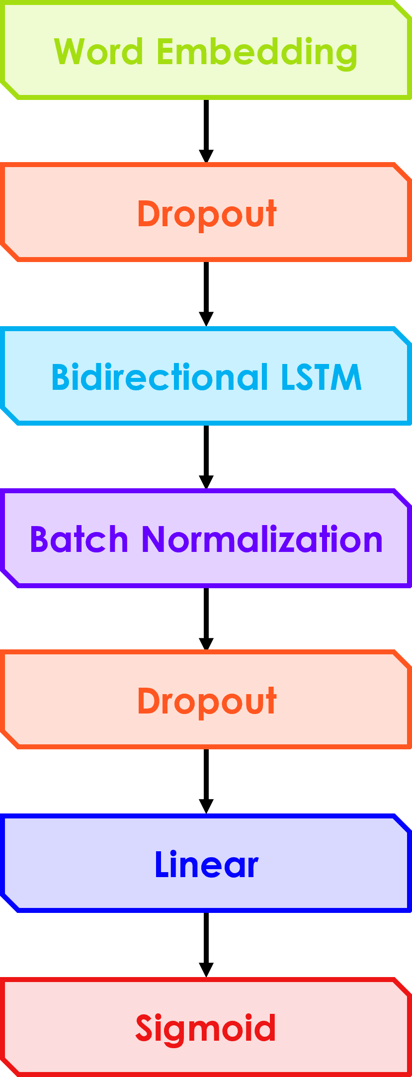
To select the best model to deploy, we each focused on different architectures, across the group covering: CNN, LSTM, transformers, SVM and One-vs-Rest classifiers. We then decided upon the bidirectional LSTM because it had a reasonably good initial performance and unlike some of the other models it is compatible with GloVe word embeddings. Through optimization, we determined the best parameters for this model were: 120 hidden layers, 70% dropout, sigmoid activation function and a batch normalization layer. The model was then integrated into a pipeline to simplify the process of training a new model trained, saving its state and automatically deploying it to our web application.

Pipeline Code

Web Application

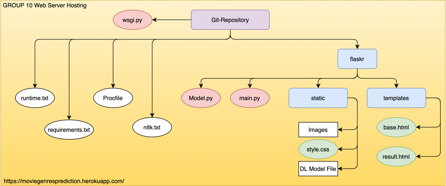
For the web application, we decided to use the Flask framework. Therefore most of the application is written in Python, apart from the front-end HTML and CSS. To restore the state of the trained LSTM, the model weights are loaded from a PyTorch file. The text pre-processor class is also loaded from a pickle file so that a description inputted by a user is processed the same way as when the model was trained.

Endpoint Functional Testing

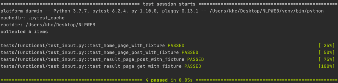
Web application unit testing are written in main.py. Functional testing was run using pytest in test_input.py to test:

GET/POST requests
Status codes of root page and result page by a built-in assertion method

Input and Prediction Monitoring

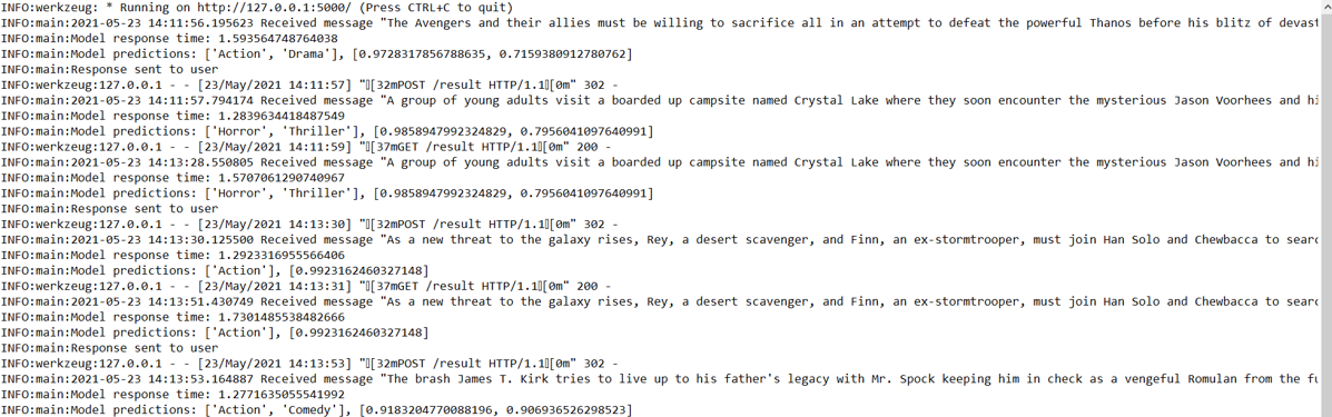
When a user input is given, the text is saved to a log file NLPWEB.log along with a time-stamp. The model's response time is recorded as well as the predicted genres and percentage confidence. The logger also documents the HTTP method and whether the server sent the prediction to the user.

Topic Modelling

An alternative approach to classification is unsupervised topic modelling approaches such as Latent Dirichlet Allocation and Latent Semantic Analysis. However, as the topics (i.e. grouping of films) uncovered by these algorithms do not align with the film's genres, they were not used to construct our final classifier.

Latent Dirichlet Allocation (LDiA)

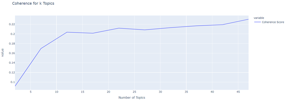
LDiA (commonly called LDA) was run on all samples to assign words into topics based on how often they occur together in a film description. As the number of topics increased, so did coherence score, i.e. the semantic similarity between high scoring words in a topic.

Figure 8a: Gensim LDiA graph of similarities and difference between topics, along with their most relevent terms

Latent Semantic Analysis (LSA)

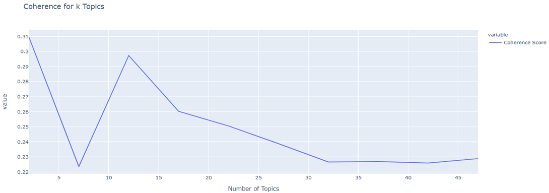
Compared to LDiA, LSA produces topics that are more spread apart in the semantic vector space. In addition, coherence score did not improve when the number of topics was increased.

Figure 9a: t-SNE graph of LDiA with 7 topics and coherence score of 0.221

Topic Modelling Code

Running the Code

The full code has been uploaded to GitHub. To download the repository, click here.

Conda Environment

To ensure all team members could execute the code during development, it was created using a conda environment. This environment has been saved as a YAML file, environment.yml, and is included in the repository. To recreate this environment, open the Anaconda prompt and enter the command below, where environment.yml is the file path of the enviroment file.

conda env create -f environment.yml

Web Application

To run the classifier web application:

conda activate MoviePredictor
Navigate to Web_App/flaskr
Run command python main.py

Jupyter Notebooks

To run the jupyter notebook(s):

conda activate MoviePredictor
Run command jupyter notebook
Upload the notebook

Contributions

Tom

CI/CD pipeline development
Model training, testing and optimization
Hosting the selected model on the backend of the web application
Creation of this site

Roger

Backend development of the Flask web application
Hosting the app prototype on Heroku
Functional testing of the application

Lavinia

Research of web service hosting options
Frontend development of the web application
Creation of video demonstrations